MULTI VARIABLE LOOPS/Advanced Type

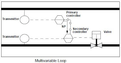
Multivariable loops are control loops in which a primary controller
controls one process variable by sending signals to a controller of a
different loop that impacts the process variable of the primary loop.
For example, the primary process variable may be the temperature of
the fluid in a tank that is heated by a steam jacket (a pressurized steam
chamber surrounding the tank). To control the primary variable
(temperature), the primary (master) controller signals the secondary
(slave) controller that is controlling steam pressure. The primary
controller will manipulate the setpoint of the secondary controller to
maintain the setpoint temperature of the primary process variable
(Figure 7.17).















When tuning a control loop, it is important to take into account the
presence of multivariable loops. The standard procedure is to tune the
secondary loop before tuning the primary loop because adjustments
to the secondary loop impact the primary loop. Tuning the primary
loop will not impact the secondary loop tuning.

FEEDFORWARD CONTROL 

Feedforward control is a control system that anticipates load
disturbances and controls them before they can impact the process
variable. For feedforward control to work, the user must have a
mathematical understanding of how the manipulated variables will
impact the process variable. Figure 7.19 shows a feedforward loop in
which a flow transmitter opens or closes a hot steam valve based on
how much cold fluid passes through the flow sensor.

An advantage of feedforward control is that error is prevented, rather
than corrected. However, it is difficult to account for all possible load
disturbances in a system through feedforward control. Factors such as
outside temperature, buildup in pipes, consistency of raw materials,
humidity, and moisture content can all become load disturbances and
cannot always be effectively accounted for in a feedforward system.
In general, feedforward systems should be used in cases where the
controlled variable has the potential of being a major load disturbance
on the process variable ultimately being controlled. The added
complexity and expense of feedforward control may not be equal to
the benefits of increased control in the case of a variable that causes
only a small load disturbance.

FEED FORWARD PLUS FEEDBACK

Because of the difficulty of accounting for every possible load
disturbance in a feedforward system, feedforward systems are often
combined with feedback systems. Controllers with summing
functions are used in these combined systems to total the input from
both the feedforward loop and the feedback loop, and send a unified
signal to the final control element. Figure 7.20 shows a
feedforward-plus-feedback loop in which both a flow transmitter and
a temperature transmitter provide information for controlling a hot
steam valve.

CASCADE CONTROL

Cascade control is a control system in which a secondary (slave)
control loop is set up to control a variable that is a major source of load
disturbance for another primary (master) control loop. The controller
of the primary loop determines the setpoint of the summing contoller in
the secondary loop (Figure 7.25).

BATCH CONTROL

Batch processes are those processes that are taken from start to finish
in batches. For example, mixing the ingredients for a juice drinks is
often a batch process. Typically, a limited amount of one flavor (e.g.,
orange drink or apple drink) is mixed at a time. For these reasons, it is
not practical to have a continuous process running. Batch processes
often involve getting the correct proportion of ingredients into the
batch. Level, flow, pressure, temperature, and often mass
measurements are used at various stages of batch processes.
A disadvantage of batch control is that the process must be frequently
restarted. Start-up presents control problems because, typically, all
measurements in the system are below setpoint at start-up. Another
disadvantage is that as recipes change, control instruments may need
to be recalibrated.

RATIO CONTROL

Imagine a process in which an acid must be diluted with water in the
proportion two parts water to one part acid. If a tank has an acid
supply on one side of a mixing vessel and a water supply on the other,
a control system could be developed to control the ratio of acid to
water, even though the water supply itself may not be controlled. This
type of control system is called ratio control (Figure 7.26). Ratio
control is used in many applications and involves a contoller that
receives input from a flow measurement device on the unregulated
(wild) flow. The controller performs a ratio calculation and signals the
appropriate setpoint to another controller that sets the flow of the
second fluid so that the proper proportion of the second fluid can be
added.
Ratio control might be used where a continuous process is going on
and an additive is being put into the flow (e.g., chlorination of water).

SELECTIVE CONTROL 

Selective control refers to a control system in which the more
important of two variables will be maintained. For example, in a
boiler control system, if fuel flow outpaces air flow, then
uncombusted fuel can build up in the boiler and cause an explosion.
Selective control is used to allow for an air-rich mixture, but never a
fuel-rich mixture. Selective control is most often used when
equipment must be protected or safety maintained, even at the cost of
not maintaining an optimal process variable setpoint.

FUZZY CONTROL

Fuzzy control is a form of adaptive control in which the controller
uses fuzzy logic to make decisions about adjusting the process.Fuzzy
logic is a form of computer logic where whether something is or is
not included in a set is based on a grading scale in which multiple
factors are accounted for and rated by the computer. The essential
idea of fuzzy control is to create a kind of artificial intelligence that
will account for numerous variables, formulate a theory of how to
make improvements, adjust the process, and learn from the result.
Fuzzy control is a relatively new technology. Because a machine
makes process control changes without consulting humans, fuzzy
control removes from operators some of the ability, but none of the
responsibility, to control a process.

Single Control Loops

PRESSURE CONTROL LOOPS

Pressure control loops vary in speed—that is, they can respond to
changes in load or to control action slowly or quickly. The speed
required in a pressure control loop may be dictated by the volume of
the process fluid. High-volume systems (e.g., large natural gas storage
facilities) tend to change more slowly than low-volume systems
(Figure 7.21).

FLOW CONTROL LOOPS

Generally, flow control loops are regarded as fast loops that respond
to changes quickly. Therefore, flow control equipment must have fast
sampling and response times. Because flow transmitters tend to be
rather sensitive devices, they can produce rapid fluctuations or noise
in the control signal. To compensate for noise, many flow transmitters
have a damping function that filters out noise. Sometimes, filters are
added between the transmitter and the control system. Because the
temperature of the process fluid affects its density, temperature
measurements are often taken with flow measurements and
compensation for temperature is accounted for in the flow
calculation. Typically, a flow sensor, a transmitter, a controller, and a
valve or pump are used in flow control loops (Figure 7.22).

LEVEL CONTROL LOOPS

The speed of changes in a level control loop largely depends on the
size and shape of the process vessel (e.g., larger vessels take longer to
fill than smaller ones) and the flow rate of the input and outflow
pipes. Manufacturers may use one of many different measurement
technologies to determine level, including radar, ultrasonic, float
gauge, and pressure measurement. The final control element in a level
control loop is usually a valve on the input and/or outflow
connections to the tank (Figure 7.23). Because it is often critical to
avoid tank overflow, redundant level control systems are sometimes
employed

TEMPERATURE CONTROL LOOPS

Because of the time required to change the temperature of a process
fluid, temperature loops tend to be relatively slow. Feedforward
control strategies are often used to increase the speed of the
temperature loop response. RTDs or thermocouples are typical
temperature sensors. Temperature transmitters and controllers are
used, although it is not uncommon to see temperature sensors wired
directly to the input interface of a controller. The final control element
for a temperature loop is usually the fuel valve to a burner or a valve
to some kind of heat exchanger. Sometimes, cool process fluid is
added to the mix to maintain temperature (Figure 7.24).

Controller Tuning

Controllers are tuned in an effort to match the characteristics of the
control equipment to the process so that two goals are achieved:
is the foundation of process control measurement in that electricity:

• The system responds quickly to errors.
• The system remains stable (PV does not oscillate around  the SP).

GAIN

Controller tuning is performed to adjust the manner in which a control

valve (or other final control element) responds to a change in error.

In particular, we are interested in adjusting the gain of the controller

such that a change in controller input will result in a change in

Gain is defined simply as the change in output divided by the change

in input.

Examples:

Change in Input to Controller - 10%

Change in Input to Controller - 10%

Change in Controller Output - 5%

Gain = 5% / 10% = 0.5

convey measurements and instructions to other instruments in a

control loop to maintain the highest level of safety and efficiency.

The next three sections in this module discuss electricity, circuits,

transmitters, and signals in greater detail so you can understand the

importance of electricity in process control.

controller output that will, in turn, cause sufficient change in

valve position to eliminate error, but not so great a change as

to cause instability or cycling.

Change in Controller Output - 20%

Gain = 20% / 10% = 2

Gain Plot - The Figure below is simply another graphical way of

representing the concept of gain.

Gain Kc =D Output % / D Input %

PROPORTIONAL ACTION

The proportional mode is used to set the basic gain value of the

controller. The setting for the proportional mode may be expressed

as either:

1. Proportional Gain

2. Proportional Band 

proportional gain. 

Proportional Gain (Kc) answers the question:

"What is the percentage change of the controller output relative to the

percentage change in controller input?"

Proportional Gain is expressed as:

Gain, (Kc) = DOutput% /DInput %

PROPORTIONAL BAND

Proportional Band (PB) is another way of representing the same

information and answers this question:

"What percentage of change of the controller input span will cause a

100% change in controller output?"

PB = DInput (% Span) For 100%DOutput

Converting Between PB and Gain

A simple equation converts gain to proportional Band:

added.

PB = 100/Gain

Also recall that:

Gain = 100%/PB

Proportional Gain, (Kc) = DOutput% / DInput %

PB= DInput(%Span) For 100%DOutput

LIMITS OF PROPORTIONAL ACTION

Responds Only to a Change in error - Proportional action responds

only to a change in the magnitude of the error.

Does Not Return the PV to Setpoint - Proportional action will not

return the PV to setpoint. It will, however, return the PV to a value

that is within a defined span (PB) around the PV.

DETERMINING THE CONTROLLER OUTPUT

Controller Output - In a proportional only controller, the output is a

function of the change in error and controller gain.

Output Change, % = (Error Change, %) (Gain)

Example: If the setpoint is suddenly changed 10% with a proportional

band setting of 50%, the output will change as follows:

Calculating Controller Output

DController Output = DInput, % X Gain

Gain = 100%/PB

EXAMPLE

DInput = 10%

PB = 50%, so Gain = 100%/50% = 2

DController Output = D Input X Gain

DController Output = 10% X 2 = 20%

Expressed in Units:

Controller Output Change = (0.2)(12 psi span) = 2.4 psi OR

(0.2)(16 mA span) = 3.2 mA

PROPORTIONAL ACTION - CLOSED LOOP

Loop Gain - Every loop has a critical or natural frequency. This is the

frequency at which cycling may exist. This critical frequency is

Low Gain Example - In the example below, the proportional band is

high (gain is low). The loop is very stable, but an error remains between

SP and PV.

determined by all of the loop components. If the loop gain is too high

at this frequency, the PV will cycle around the SP; i.e., the process

will become unstable.

High Gain Example - In the example, the proportional band is

small resulting in high gain, which is causing instability. Notice that

the process variable is still not on set point.

Proportional Summary - For the proportional mode, controller output

is a function of a change in error. Proportional band is expressed in

terms of the percentage change in error that will cause 100% change in

controller output. Proportional gain is expressed as the percentage

change in output divided by the percentage change in input.

PB = (DInput, % / DOutput, % ) x 100 = 100/Gain

Gain= DInput % / DOutput %

D Controller Output = (Change in Error)(Gain)

1. Proportional Mode Responds only to a change in error

2. Proportional mode alone will not return the PV to SP.

Advantages - Simple

Disadvantages - Error

Settings - PB settings have the following effects:

Small PB (%) Minimize Offset

High Gain (%) Possible cycling

Large PB (%) Large Offset

Low Gain Stable Loop

Tuning - reduce PB (increase gain) until the process cycles following

a disturbance, then double the PB (reduce gain by 50%).

INTEGRAL ACTION

Duration of Error and Integral Mode - Another component of error 

is the duration of the error, i.e., how long has the error existed? 

The controller output from the integral or reset mode is a function of

the duration of the error.

OPEN LOOP ANALYSIS

Purpose- The purpose of integral action is to return the PV to SP. This is

accomplished by repeating the action of the proportional mode as

long as an error exists. With the exception of some electronic

controllers, the integral or reset mode is always used with the

proportional mode.

Setting - Integral, or reset action, may be expressed in terms of:

Repeats Per Minute - How many times the proportional

action is repeated each minute.

Minutes Per Repeat - How many minutes are required for

1 repeat to occur.

CLOSED LOOP ANALYSIS
Closed Loop With Reset - Adding reset to the controller adds one more

gain component to the loop. The faster the reset action, the greater
the gain.
Slow Reset Example - In this example the loop is stable because
the total loop gain is not too high at the loop critical frequency.
Notice that the process variable does reach set point due to the reset
action.

RESETWINDUP
Defined - Reset windup is described as a situation where the controller
output is driven from a desired output level because of a large
difference between the set point and the process variable.

Shutdown - Reset windup is common on shut down because the
process variable may go to zero but the set point has not changed,
therefore this large error will drive the output to one extreme.

Startup - At start up, large process variable overshoot may occur
because the reset speed prevents the output from reaching its desired
value fast enough.
Anti Reset Windup - Controllers can be modified with an anti-reset
windup (ARW) device. The purpose of an anti-reset option is to allow
the output to reach its desired value quicker, therefore minimizing
the overshoot.
Fast Reset (Large Repeats/Min.,Small Min./Repeat)
 1.High Gain
2.Fast Return To Setpoint
3.Possible Cycling
Slow Reset(Small Repeats/Min.,Large Min./Repeats)
 1.Low Gain
2.Slow Return To Setpoint
3.Stable Loop
Trailing and Error Tuning - Increase repeats per minute until the
PV cycles following a disturbance, then slow the reset action to a
value that is 1/3 of the initial setting.
SUMMARY
Integral (Reset) Summary - Output is a repeat of the proportional
action as long as error exists. The units are in terms of repeats per
minute or minutes per repeat.
Advantages - Eliminates error
Disadvantages - Reset windup and possible overshoot

DERIVATIVE ACTION
Derivative Mode Basics - Some large and/or slow process do not
The derivative action is initiated whenever there is a change in the
rate of change of the error (the slope of the PV). The magnitude of
the derivative action is determined by the setting of the derivative . The
respond well to small changes in controller output. For example,
a large liquid level process or a large thermal
process (a heat exchanger) may react very slowly to a small change
in controller output. To improve response, a large initial change in
controller output may be applied. This action is the role of the
derivative mode.
mode of a PID controller and the rate of change of the PV. The
Derivative setting is expressed in terms of minutes. In oper ation, the
the controller first compares the current PV with the last value of the
PV. If there is a change in the slope of the PV, the controller
etermines what its output would be at a future point in time
(the future point in time is determined by the value of the derivative
setting, in minutes). The derivative mode immediately increases
the output by that amount.

Example - Let's start a closed loop example by looking at a
temperature control system. IN this example, the time scale has been
lengthened to help illustrate controller actions in a slow process.
Rate Effect - To illustrate the effect of rate action, we will add the
are mode with a setting of 1 minute. Notice the very large controller
output at time 0. The output spike is the result of rate action. Recall
Assume a proportional band settingof 50%. There is no reset at
this time. The proportional gain of 2 acting on a 10% change in set
pint results in a change in controller output of 20%. Because
temperature is a slow process the setting time after a change in error
is quite long. And, in this example, the PV never becomes equal to
the SP because there is no reset.
that the change in output due to rate action is a function of the speed
(rate) of change of error, which in a step is nearly infinite. The
addition of rate alone will not cause the process variable to match the
set point.

Effect of Fast Rate - Let's now increase the rate setting to 10 minutes.
The controller gain is now much higher. As a result, both the IVP
(controller output) and the PV are cycling. The point here is that
increasing the rate setting will not cause the PV to settle at the SP.

Need for Reset Action - It is now clear that reset must be added to
bring process variable back to set point
Applications - Because this component of the controller output is
dependent on the speed of change of the input or error, the output
will be very erratic if rate is used on fast process or one with noisy
signals. The controller output, as a result of rate, will have the
greatest change when the input changes rapidly.
Controller Option to Ignore Change in SP - Many controllers,
especially digital types, are designed to respond to changes in the PV
only, and to ignore changes in SP. This feature eliminates a major upset
upset that would occur following a change in the setpoint.

SUMMARY
Derivative (Rate) Sumary - Rate action is a function of the speed of
change of the error. The units are minutes. The action is to apply an
immediate response that is equal to the proportional plus reset action
that would have occurred some number of minutes I the future.

Advantages - Rapid output reduces the time that is required to return
PV to SP in slow process.
Disadvantage - Dramatically amplifies noisy signals; can cause
cycling in fast processes.
Settings
Large (Minutes)
 1.High Gain
2.Large Output Change
3.Possible Cycling
Small (Minutes)
 1.Low Gain
2.Small Output Change
3.Stable Loop
Trial-and-Error Tuning
Increase the rate setting until the process cycles following a
disturbance, then reduce the rate setting to one-third of the initial
value.

Controllers

The actions of controllers can be divided into groups based upon the
functions of their control mechanism. Each type of contoller has
advantages and disadvantages and will meet the needs of different
applications. Grouped by control mechanism function, the three
types of controllers are:

• Discrete controllers
• Multistep controllers
• Continuous controllers

DISCRETE CONTROLLERS
Discrete controllers are controllers that have only two modes or
positions: on and off. A common example of a discrete controller is a
home hot water heater. When the temperature of the water in the tank
falls below setpoint, the burner turns on. When the water in the tank
reaches setpoint, the burner turns off. Because the water starts
cooling again when the burner turns off, it is only a matter of time
before the cycle begins again. This type of control doesn’t actually
hold the variable at setpoint, but keeps the variable within proximity
of setpoint in what is known as a dead zone (Figure 7.15).

MULTISTEP CONTROLLERS


Multistep controllers are controllers that have at least one other
possible position in addition to on and off. Multistep controllers
operate similarly to discrete controllers, but as setpoint is approached,
the multistep controller takes intermediate steps. Therefore, the
oscillation around setpoint can be less dramatic when multistep
controllers are employed than when discrete controllers are used
(Figure 7.16).















CONTINUOUS CONTROLLERS

Controllers automatically compare the value of the PV to the SP to
determine if an error exists. If there is an error, the controller adjusts
its output according to the parameters that have been set in the
controller. The tuning parameters essentially determine:
How much correction should be made? The magnitude of the
correction( change in controller output) is determined by the
proportional mode of the controller.
How long should the correction be applied? The duration of the
adjustment to the controller output is determined by the integral mode
of the controller
How fast should the correction be applied? The speed at which a
correction is made is determined by the derivative mode of the
controller.

ISA Standards Symbology

The Instrumentation, Systems, and Automation Society (ISA) is one of
the leading process control trade and standards organizations. The ISA
has developed a set of symbols for use in engineering drawings and
designs of control loops (ISA S5.1 instrumentation symbol
specification). You should be familiar with ISA symbology so that you
can demonstrate possible process control loop solutions on paper to
your customer.


IDENTIFICATION LETTERS
Identification letters on the ISA symbols (e.g., TT for temperature
transmitter) indicate:
The variable being measured (e.g., flow, pressure, temperature)
The device’s function (e.g., transmitter, switch, valve, sensor,
indicator)
Some modifiers (e.g., high, low, multifunction)
Table 7.1 on page 26 shows the ISA identification letter designations.
The initial letter indicates the measured variable. The second letter
indicates a modifier, readout, or device function. The third letter
usually indicates either a device function or a modifier.
For example, “FIC” on an instrument tag represents a flow indicating
controller. “PT” represents a pressure transmitter. You can find
identification letter symbology information on the ISA Web site at
http://www.isa.org.

TAG NUMBERS
Numbers on P&ID symbols represent instrument tag numbers. Often
these numbers are associated with a particular control loop

Figure 7.5 shows a control loop using ISA symbology.
Drawings of this kind are known as piping and instrumentation
drawings (P&ID).












SYMBOLS

In a P&ID, a circle represents individual measurement instruments,
such as transmitters, sensors, and detectors (Figure 7.6).
A single horizontal line running across the center of the shape
indicates that the instrument or function is located in a primary
location (e.g., a control room). A double line indicates that the
function is in an auxiliary location (e.g., an instrument rack). The
absence of a line indicates that the function is field mounted, and a
dotted line indicates that the function or instrument is inaccessible
(e.g., located behind a panel board).
A square with a circle inside represents instruments that both display
measurement readings and perform some control function
(Figure 7.7). Many modern transmitters are equipped with
microprocessors that perform control calculations and send control
output signals to final control elements.

Piping and Connections

Piping and connections are represented with several different symbols

Components of Control Loops

This section describes the instruments, technologies, and equipment used to develop and maintain process
control loops. In addition, this section describes how process control equipment is represented in technical
drawings of control loops.

PRIMARY ELEMENTS/SENSORS
In all cases, some kind of instrument is measuring changes in the
process and reporting a process variable measurement. Some of the
greatest ingenuity in the process control field is apparent in sensing
devices. Because sensing devices are the first element in the control
loop to measure the process variable, they are also called primary
elements. Examples of primary elements include:

• Pressure sensing diaphragms, strain gauges, capacitance cells
• Resistance temperature detectors (RTDs)
• Thermocouples
• Orifice plates
• Pitot tubes
• Venturi tubes
• Magnetic flow tubes
• Coriolis flow tubes
• Radar emitters and receivers
• Ultrasonic emitters and receivers
• Annubar flow elements
• Vortex sheddar

Primary elements are devices that cause some change in their
property with changes in process fluid conditions that can then be
measured. For example, when a conductive fluid passes through the
magnetic field in a magnetic flow tube, the fluid generates a voltage
that is directly proportional to the velocity of the process fluid. The
primary element (magnetic flow tube) outputs a voltage that can be
measured and used to calculate the fluid’s flow rate. With an RTD, as
the temperature of a process fluid surrounding the RTD rises or falls,
the electrical resistance of the RTD increases or decreases a
proportional amount. The resistance is measured, and from this
measurement, temperature is determined.

TRANSDUCERS AND CONVERTERS
Activities
A transducer is a device that translates a mechanical signal into an
electrical signal. For example, inside a capacitance pressure device, a
transducer converts changes in pressure into a proportional change in
capacitance.
A converter is a device that converts one type of signal into another
type of signal. For example, a converter may convert current into
voltage or an analog signal into a digital signal. In process control, a
converter used to convert a 4–20 mA current signal into a 3–15 psig
pneumatic signal (commonly used by valve actuators) is called a
current-to-pressure converter.
TRANSMITTERS
A transmitter is a device that converts a reading from a sensor
or transducer into a standard signal and transmits that signal
to a monitor or controller. Transmitter types include:

•  Pressure transmitters
•  Flow transmitters
•  Temperature transmitters
•  Level transmitters
•  Analytic (O2 [oxygen], CO [carbon monoxide], and pH)

transmitters

Process Signals

SIGNALS
There are three kinds of signals that exist for the process industry to
transmit the process variable measurement from the instrument to a
centralized control system.
1. Pneumatic signal
2. Analog signal
3. Digital signal





Pneumatic Signals
Pneumatic signals are signals produced by changing the air pressure
in a signal pipe in proportion to the measured change in a process
variable. The common industry standard pneumatic signal range is
3–15 psig. The 3 corresponds to the lower range value (LRV) and the
15 corresponds to the upper range value (URV). Pneumatic signalling
is still common. However, since the advent of electronic instruments
in the 1960s, the lower costs involved in running electrical signal wire
through a plant as opposed to running pressurized air tubes has made
pneumatic signal technology less attractive.

Analog Signals
The most common standard electrical signal is the 4–20 mA current
signal. With this signal, a transmitter sends a small current through a
set of wires. The current signal is a kind of gauge in which
4 mA represents the lowest possible measurement, or zero, and 20
mA represents the highest possible measurement.
For example, imagine a process that must be maintained at 100 °C.
An RTD temperature sensor and transmitter are installed in the
process vessel, and the transmitter is set to produce a 4 mA signal
when the process temperature is at 95 °C and a 20 mA signal
when the process temperature is at 105 °C. The transmitter will
transmit a 12 mA signal when the temperature is at the 100 °C
setpoint. As the sensor’s resistance property changes in
response to changes in temperature, the transmitter outputs a
4–20 mA signal that is proportionate to the temperature changes. This
signal can be converted to a temperature reading or an
input to a control device, such as a burner fuel valve.
Other common standard electrical signals include the 1–5 V (volts)
signal and the pulse output.

Digital Signals
Digital signals are the most recent addition to process control signal
technology. Digital signals are discrete levels or values that are
combined in specific ways to represent process variables and also carry
other information, such as diagnostic information. The methodology
used to combine the digital signals is referred to as protocol.
Manufacturers may use either an open or a proprietary digital
protocol. Open protocols are those that anyone who is developing a
control device can use. Proprietary protocols are owned by specific
companies and may be used only with their permission. Open digital
protocols include the HART® (highway addressable remote
transducer) protocol, FOUNDATION™ Fieldbus, Profibus, DeviceNet,
and the Modbus® protocol.
(See Module 8: Communication Technologies for more information
on digital communication protocols.)

Process Variables

SETPOINT
The setpoint is a value for a process variable that is desired to be
maintained. For example, if a process temperature needs to kept
within 5 °C of 100 °C, then the setpoint is 100 °C. A temperature
sensor can be used to help maintain the temperature at setpoint.
The sensor is inserted into the process, and a contoller compares the
temperature reading from the sensor to the setpoint. If the temperature
reading is 110 °C, then the controller determines that the process is
above setpoint and signals the fuel valve of the burner to close slightly
until the process cools to 100 °C. Set points can also be maximum or
minimum values. For example, level in tank cannot exceed 20 feet.

MEASURED VARIABLES, PROCESS VARIABLES, AND
MANIPULATED VARIABLES
In the temperature control loop example, the measured variable is
temperature, which must be held close to 100 °C. In this example and
in most instances, the measured variable is also the process variable.
The measured variable is the condition of the process fluid that must
be kept at the designated setpoint.
Sometimes the measured variable is not the same as the process
variable. For example, a manufacturer may measure flow into and out
of a storage tank to determine tank level. In this scenario, flow is the
measured variable, and the process fluid level is the process variable.
The factor that is changed to keep the measured variable at setpoint is
called the manipulated variable. In the example described, the
manipulated variable would also be flow.

ERROR
Error is the difference between the measured variable and the
setpoint and can be either positive or negative. In the temperature
control loop example, the error is the difference between the 110 °C
measured variable and the 100 °C setpoint—that is, the error is +10
°C.
The objective of any control scheme is to minimize or eliminate error.
Therefore, it is imperative that error be well understood. Any error
can be seen as having three major components. These three
components are shown in the figure on the folowing page
Magnitude
The magnitude of the error is simply the deviation between the values
of the setpoint and the process variable. The magnitude of error at any
point in time compared to the previous error provides the basis for
determining the change in error. The change in error is also an
important value.

Duration
Duration refers to the length of time that an error condition has
existed.
Rate Of Change
The rate of change is shown by the slope of the error plot.

OFFSET
Offset is a sustained deviation of the process variable from the
setpoint. In the temperature control loop example, if the control
system held the process fluid at 100.5 °C consistently, even though
the setpoint is 100 °C, then an offset of 0.5 °C exists.
LOAD DISTURBANCE
A load disturbance is an undesired change in one of the factors that
can affect the process variable. In the temperature control loop
example, adding cold process fluid to the vessel would be a load
disturbance because it would lower the temperature of the process
fluid.
CONTROL ALGORITHM
A control algorithm is a mathematical expression of a control
function. Using the temperature control loop example, V in the
equation below is the fuel valve position, and e is the error. The
relationship in a control algorithm can be expressed as:
The fuel valve position (V) is a function (f) of the sign (positive or
negative) of the error (Figure 7.3).
Algorithm Example
Control algorithms can be used to calculate the requirements of much
more complex control loops than the one described here. In more
complex control loops, questions such as “How far should the valve
be opened or closed in response to a given change in setpoint?” and
“How long should the valve be held in the new position after the
process variable moves back toward setpoint?” need to be answered.
MANUAL AND AUTOMATIC CONTROL
Before process automation, people, rather than machines, performed
many of the process control tasks. For example, a human operator
might have watched a level gauge and closed a valve when the level
reached the setpoint. Control operations that involve human
action to make an adjustment are called manual control systems.
Conversely, control operations in which no human intervention is
required, such as an automatic valve actuator that responds to a level
controller, are called automatic control systems.
V = f(± e)

Control algorithms can be used to calculate the requirements of much
more complex control loops than the one described here. In more
complex control loops, questions such as “How far should the valve
be opened or closed in response to a given change in setpoint?” and
“How long should the valve be held in the new position after the
process variable moves back toward setpoint?” need to be answered.

PROCESS VARIABLE

A process variable is a condition of the process fluid (a liquid or gas)
that can change the manufacturing process in some way. In the example of you sitting by the fire, the process variable was temperature. In the example of the tank in Figure 7.1, the process variable is level. Common process variables include:

• Pressure
• Flow
• Level
• Temperature
• Density
• Ph (acidity or alkalinity)
• Liquid interface (the relative amounts of different liquids that are combined in a vessel)
• Mass
• Conductivity

The Control Loop

Imagine you are sitting in a cabin in front of a small fire on a cold
winter evening. You feel uncomfortably cold, so you throw another
log on the fire. Thisis an example of a control loop. In the
control loop, a variable (temperature) fell below the setpoint (your
comfort level), and you took action to bring the process back into the
desired condition by adding fuel to the fire. The control loop will
now remain static until the temperature

Control loops in the process control industry work in the same way,
requiring three tasks to occur:

• Measurement
• Comparison
• Adjustment

In Figure 7.1, a level transmitter (LT) measures the level in the tank
and transmits a signal associated with the level reading to a controller
(LIC). The controller compares the reading to a predetermined value,
in this case, the maximum tank level established by the plant
operator, and finds that the values are equal. The controller then
sends a signal to the device that can bring the tank level back to a
lower level—a valve at the bottom of the tank. The valve opens to let
some liquid out of the tank.
Many different instruments and devices may or may not be used in
control loops (e.g., transmitters, sensors, controllers, valves, pumps),
but the three tasks of measurement, comparison, and adjustment are
always present.

The Importance of Process Control

Refining, combining, handling, and otherwise manipulating fluids to profitably produce end products can be a
precise, demanding, and potentially hazardous process. Small changes in a process can have a large impact
on the end result. Variations in proportions, temperature, flow, turbulence, and many other factors must be
carefully and consistently controlled to produce the desired end product with a minimum of raw materials and
energy. Process control technology is the tool that enables manufacturers to keep their operations running
within specified limits and to set more precise limits to maximize profitability, ensure quality and safety.

Process as used in the terms process control and process industry,
refers to the methods of changing or refining raw materials to create
end products. The raw materials, which either pass through or remain
in a liquid, gaseous, or slurry (a mix of solids and liquids) state
during the process, are transferred, measured, mixed, heated or
cooled, filtered, stored, or handled in some other way to produce the
end product.
Process industries include the chemical industry, the oil and gas
industry, the food and beverage industry, the pharmaceutical industry,
the water treatment industry, and the power industry.

Reducing variability can also save money by reducing the need for Activities
product padding to meet required product specifications. Padding
refers to the process of making a product of higher-quality than it
needs to be to meet specifications. When there is variability in the end
product (i.e., when process control is poor), manufacturers are forced
to pad the product to ensure that specifications are met, which adds
to the cost. With accurate, dependable process control, the setpoint
(desired or optimal point) can be moved closer to the actual product
specification and thus save the manufacturer money.

Manufacturers control the production process for
three reasons:

1. Reduce variability
2. Increase efficiency
3. Ensure safety

• Reduce Variability

Process control can reduce variability in the end product, which
ensures a consistently high-quality product. Manufacturers can also
save money by reducing variability. For example, in a gasoline
blending process, as many as 12 or more different components
may be blended to make a specific grade of gasoline. If the refinery
does not have precise control over the flow of the separate
components, the gasoline may get too much of the high-octane
components. As a result, customers would receive a higher grade
and more expensive gasoline than they paid for, and the refinery
would lose money. The opposite situation would be customers
receiving a lower grade at a higher price.

• Increase Efficiency

Some processes need to be maintained at a specific point to maximize
efficiency. For example, a control point might be the temperature at
which a chemical reaction takes place. Accurate control of temperature
ensures process efficiency. Manufacturers save money by minimizing
the resources required to produce the end product.

• Ensure Safety

A run-away process, such as an out-of-control nuclear or chemical
reaction, may result if manufacturers do not maintain precise control
of all of the processg variables. The consequences of a run-away
process can be catastrophic.
Precise process control may also be required to ensure safety. For
example, maintaining proper boiler pressure by controlling the inflow
of air used in combustion and the outflow of exhaust gases is crucial
in preventing boiler implosions that can clearly threaten the safety of
workers.

Introduction To Process Control

Control in process industries refers to the regulation of all aspects of the process. Precise control of level,
temperature, pressure and flow is important in many process applications.

Process control refers to the methods that are used to control process
variables when manufacturing a product. For example, factors such
as the proportion of one ingredient to another, the temperature of the
materials, how well the ingredients are mixed, and the pressure under
which the materials are held can significantly impact the quality of
an end product.

VFD- VFD OPERATION

Understanding the basic principles behind VFD operation requires understanding the three basic sections of the VFD: the rectifier, dc bus, and inverter.
The voltage on an alternating current (ac) power supply rises and falls in the pattern of a sine wave
(see Figure 1). When the voltage is positive, current
flows in one direction; when the voltage is negative,
the current flows in the opposite direction. This type
of power system enables large amounts of energy to
be efficiently transmitted over great distances             .
The rectifier in a VFD is used to convert incoming
ac power into direct current (dc) power. One rectifier
 will allow power to pass through only when the
voltage is positive. A second rectifier will allow
power to pass through only when the voltage is negative.
 Two rectifiers are required for each phase of
power. Since most large power supplies are three
phase, there will be a minimum of 6 rectifiers used
(see Figure 2). Appropriately, the term “6 pulse” is
used to describe a drive with 6 rectifiers. A VFD
may have multiple rectifier sections, with 6 rectifiers per section, enabling a VFD to be “12 pulse,”
“18 pulse,” or “24 pulse.” The benefit of “multipulse” VFDs will be described later in the harmonics section.
Rectifiers may utilize diodes, silicon controlled rectifiers (SCR), or transistors to rectify power. Diodes
are the simplest device and allow power to flow any
time voltage is of the proper polarity. Silicon controlled rectifiers include a gate circuit that enables a
microprocessor to control when the power may
begin to flow, making this type of rectifier useful for
solid-state starters as well. Transistors include a gate
circuit that enables a microprocessor to open or
close at any time, making the transistor the most
useful device of the three. A VFD using transistors
in the rectifier section is said to have an “active
front end.”
After the power flows through the rectifiers it is
stored on a dc bus. The dc bus contains capacitors
to accept power from the rectifier, store it, and later
deliver that power through the inverter section. The
dc bus may also contain inductors, dc links, chokes,
or similar items that add inductance, thereby
smoothing the incoming power supply to the dc bus.
The final section of the VFD is referred to as an
“inverter.” The inverter contains transistors that
deliver power to the motor. The “Insulated Gate
Bipolar Transistor” (IGBT) is a common choice in
modern VFDs. The IGBT can switch on and off several thousand times per second and precisely control
the power delivered to the motor. The IGBT uses a
method named “pulse width modulation” (PWM)
to simulate a current sine wave at the desired frequency to the motor.
Motor speed (rpm) is dependent upon frequency.
Varying the frequency output of the VFD controls
motor speed:
Speed (rpm) = frequency (hertz) x 120 / no. of poles

Variable Frequency Drives (VFD)

A variable-frequency drive (VFD) (also termed adjustable-frequency drive, variable-speed drive, AC drive, micro drive or inverter drive) is a type of adjustable-speed drive used in electro-mechanical drive systems to control AC motor speed and torque by varying motor input frequency and voltage.

VFDs are used in applications ranging from small appliances to the largest of mine mill drives and compressors. However, about a third of the world's electrical energy is consumed by electric motors in fixed-speed centrifugal pump, fan and compressor applications and VFDs' global market penetration for all applications is still relatively small. This highlights especially significant energy efficiency improvement opportunities for retrofitted and new VFD installations.

Over the last four decades, power electronics technology has reduced VFD cost and size and improved performance through advances in semiconductor switching devices, drive topologies, simulation and control techniques, and control hardware and software.

VFDs are available in a number of different low and medium voltage AC-AC and DC-AC topologies

What is a Relay

         A relay is an electrically operated switch. Many relays use an electromagnet to operate a switching mechanism mechanically, but other operating principles are also used. Relays are used where it is necessary to control a circuit by a low-power signal (with complete electrical isolation between control and controlled circuits), or where several circuits must be controlled by one signal. The first relays were used in long distance telegraph circuits, repeating the signal coming in from one circuit and re-transmitting it to another. Relays were used extensively in telephone exchanges and early computers to perform logical operations.

A type of relay that can handle the high power required to directly control an electric motor or other loads is called a contactor. Solid-state relays control power circuits with no moving parts, instead using a semiconductor device to perform switching. Relays with calibrated operating characteristics and sometimes multiple operating coils are used to protect electrical circuits from overload or faults; in modern electric power systems these functions are performed by digital instruments still called "protective relays".

Rotary Encoder

A rotary encoder, also called a shaft encoder, is an electro-mechanical device that converts the angular position or motion of a shaft or axle to an analog or digital code.

There are two main types: absolute and incremental (relative). The output of absolute encoders indicates the current position of the shaft, making them angle transducers. The output of incremental encoders provides information about the motion of the shaft, which is typically further processed elsewhere into information such as speed, distance, and position.